Як витягти всі записи між двома датами в Excel?
Ось діапазон даних в Excel, і в цьому випадку я хочу витягти всі записи рядків між двома датами, як показано на скріншоті нижче, чи є у вас ідеї для швидкої роботи з цією роботою, не шукаючи дані та не витягуючи їх по черзі вручну?
 |
 |
Витягніть усі записи між двома датами за формулами
Витягніть усі записи між двома датами за допомогою Kutools для Excel![]()
Витягніть усі записи між двома датами за формулами

Щоб витягти всі записи між двома датами в Excel, потрібно виконати такі дії:
1. Створіть новий аркуш, Аркуш2, і введіть дату початку та дату закінчення у дві клітинки, наприклад, А1 та В1. Дивіться знімок екрана:
2. У C1 на аркуші2 введіть цю формулу, =SUMPRODUCT((Sheet1!$A$2:$A$22>=A2)*(Sheet1!$A$2:$A$22<=B2)), натисніть
Що натомість? Створіть віртуальну версію себе у
для підрахунку загальної кількості відповідних рядків. Дивіться знімок екрана: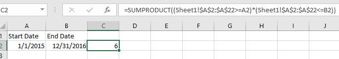
Примітка: у формулі Аркуш1 - аркуш містить вихідні дані, з яких потрібно витягти, $ A $ 2: $ A $ 22 - діапазон даних, A2 і B2 - дата початку та дата закінчення.
3. Виділіть порожню комірку, куди ви розмістите витягнуті дані, введіть цю формулу =IF(ROWS(A$5:A5)>$C$2,"",INDEX(Sheet1!A$2:A$22,SMALL(IF((Sheet1!$A$2:$A$22>=$A$2)*(Sheet1!$A$2:$A$22<=$B$2),ROW(Sheet1!A$2:A$22)-ROW(Sheet1!$A$2)+1),ROWS(A$5:A5)))), натисніть Shift + Ctrl + Enter клавіші та перетягніть маркер автоматичного заповнення по стовпцях і рядках, щоб витягти всі дані, поки не з’являться порожні комірки або нульові значення. Дивіться знімок екрана:
4. Видаліть нулі та виберіть дати, що відображаються як 5-значні числа, перейдіть до Головна Вкладка і виберіть Коротке побачення у розкривному списку Загальне, щоб відформатувати їх у форматуванні дати. Дивіться знімок екрана: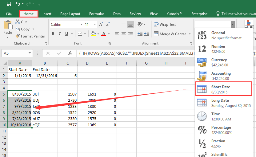
Витягніть усі записи між двома датами за допомогою Kutools для Excel
Якщо ви хочете легше впоратися з цією роботою, ви можете спробувати функцію «Вибрати конкретні клітинки» Kutools для Excel.
| Kutools для Excel, з більш ніж 300 зручні функції, полегшує вам роботу. |
після установки Kutools для Excel, виконайте наведені нижче дії.(Безкоштовно завантажте Kutools для Excel зараз!)
1. Виберіть дані, з яких ви хочете витягти, натисніть Кутулс > Select > Виберіть певні клітини. Дивіться знімок екрана:
2 В Виберіть певні клітини діалогове вікно, перевірте Весь ряд опція та виберіть Більш чим та Менш зі спадних списків введіть дату початку та дату закінчення в текстові поля, не забудьте перевірити і. Дивіться знімок екрана: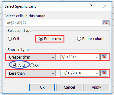
3. клацання Ok > OK. І вибрано рядки, що відповідають датам. Натисніть Ctrl + C щоб скопіювати рядки, виберіть порожню клітинку та натисніть Ctrl + V щоб вставити його, див. знімок екрана:
Демонстрація
Найкращі інструменти продуктивності офісу
Покращуйте свої навички Excel за допомогою Kutools для Excel і відчуйте ефективність, як ніколи раніше. Kutools для Excel пропонує понад 300 додаткових функцій для підвищення продуктивності та економії часу. Натисніть тут, щоб отримати функцію, яка вам найбільше потрібна...
")
Вкладка Office Передає інтерфейс із вкладками в Office і значно полегшує вашу роботу
- Увімкніть редагування та читання на вкладках у Word, Excel, PowerPoint, Publisher, Access, Visio та Project.
- Відкривайте та створюйте кілька документів на нових вкладках того самого вікна, а не в нових вікнах.
- Збільшує вашу продуктивність на 50% та зменшує сотні клацань миші для вас щодня!
")