Перейти до основного матеріалу

Як підсумувати на основі критеріїв стовпців і рядків у Excel? 

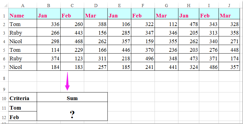
У мене є ряд даних, які містять заголовки рядків і стовпців, тепер я хочу взяти суму комірок, які відповідають критеріям заголовків стовпців і рядків. Наприклад, для підсумовування комірок, критеріями стовпців яких є Том, а критеріями рядків - лютий, як показано на наступному знімку екрана. У цій статті я розповім про деякі корисні формули для її вирішення.

критерії рядка стовпця суми документа 1

Підсумуйте комірки на основі критеріїв стовпців і рядків із формулами


стрілка синя права міхур Підсумуйте комірки на основі критеріїв стовпців і рядків із формулами

Тут ви можете застосувати наступні формули для підсумовування комірок на основі як критеріїв стовпців, так і рядків, будь ласка, зробіть так:

Введіть будь-яку з наведених нижче формул у порожню комірку, куди потрібно вивести результат:

=SUMPRODUCT((A2:A7="Tom")*(B1:J1="Feb")*(B2:J7))

=SUM(IF(B1:J1="Feb",IF(A2:A7="Tom",B2:J7)))

А потім натисніть Shift + Ctrl + Enter клавіші разом, щоб отримати результат, див. скріншот:

критерії рядка стовпця суми документа 2

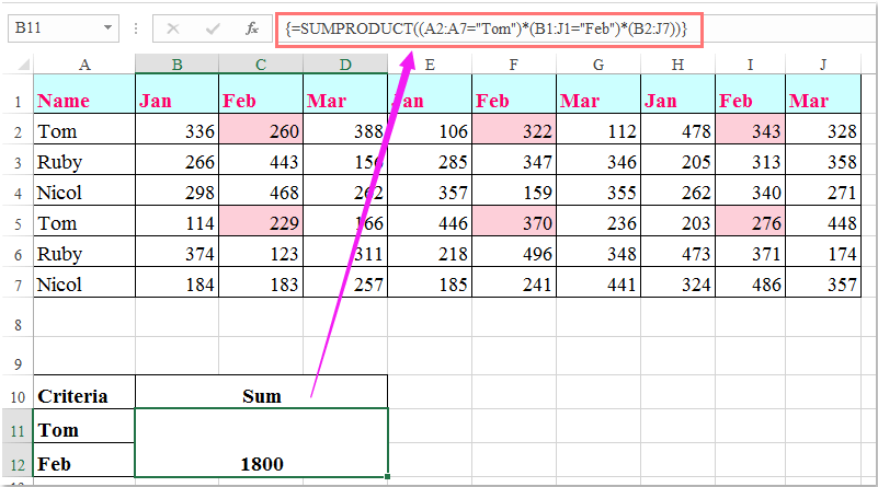
примітки: У наведених формулах: Том та Feb є критеріями стовпців і рядків, які базуються на, A2: A7, B1: J1 - заголовки стовпців і заголовки рядків містять критерії, B2: J7 - діапазон даних, який потрібно підсумувати.

Найкращі інструменти продуктивності офісу

🤖 Kutools AI Aide: Революціонізуйте аналіз даних на основі: Інтелектуальне виконання   |  Згенерувати код  |  Створення спеціальних формул  |  Аналізуйте дані та створюйте діаграми  |  Викликати функції Kutools...
Популярні функції: Знайдіть, виділіть або визначте дублікати   |  Видалити порожні рядки   |  Об’єднайте стовпці або клітинки без втрати даних   |   Раунд без Формули ...
Супер пошук: VLookup за кількома критеріями    Багатозначний VLookup  |   VLookup на кількох аркушах   |   Нечіткий пошук ....
Розширений розкривний список: Швидке створення випадаючого списку   |  Залежний спадний список   |  Виберіть розкривний список, що вибирається ....
Менеджер колонок: Додайте конкретну кількість стовпців  |  Перемістити стовпці  |  Перемкнути статус видимості прихованих стовпців  |  Порівняйте діапазони та стовпці ...
Особливості: Фокус сітки   |  Перегляд дизайну   |   Велика панель формул    Диспетчер робочих книг і аркушів   |  Бібліотека ресурсів (автотекст)   |  Вибір дати   |  Об’єднайте робочі аркуші   |  Шифрування/розшифрування клітинок    Надсилайте листи за списком   |  Супер фільтр   |   Спеціальний фільтр (фільтр жирний/курсив/закреслений...) ...
Топ-15 наборів інструментів12 текст Tools (додати текст, Видалити символи, ...)   |   50 + Графік типи (діаграма Ганта, ...)   |   40+ Практичний Формули (Розрахуйте вік на основі дня народження, ...)   |   19 вставка Tools (Вставте QR-код, Вставити зображення зі шляху, ...)   |   12 Перетворення Tools (Числа до слів, Валютна конверсія, ...)   |   7 Злиття та розділення Tools (Розширені комбіновані ряди, Розділені клітини, ...)   |   ... і більше

Покращуйте свої навички Excel за допомогою Kutools для Excel і відчуйте ефективність, як ніколи раніше. Kutools для Excel пропонує понад 300 додаткових функцій для підвищення продуктивності та економії часу.  Натисніть тут, щоб отримати функцію, яка вам найбільше потрібна...

Опис


Вкладка Office Передає інтерфейс із вкладками в Office і значно полегшує вашу роботу

  • Увімкніть редагування та читання на вкладках у Word, Excel, PowerPoint, Publisher, Access, Visio та Project.
  • Відкривайте та створюйте кілька документів на нових вкладках того самого вікна, а не в нових вікнах.
  • Збільшує вашу продуктивність на 50% та зменшує сотні клацань миші для вас щодня!
Comments (17)
No ratings yet. Be the first to rate!
This comment was minimized by the moderator on the site
Brilliant!

The function =SUM(IF(B1:J1="Feb",IF(A2:A7="Tom",B2:J7))) is a great X & Y summation tool.
I would not have thought this logic out on my own.
In fact i took me a minute to deconstruction the operations.

Thank you
This comment was minimized by the moderator on the site
My data that I am trying to retrieve is in a table. Would this impact the result at all? I have:

=SUM(IF('[Primary Controller Active Project Database (KC notes)1.xlsx]Active Project Tracking'!$B2:$B66=X2,IF('[Primary Controller Active Project Database (KC notes)1.xlsx]Active Project Tracking'!$A1:$AV1=AH10,'[Primary Controller Active Project Database (KC notes)1.xlsx]Active Project Tracking'!$H$2:$AV$66)))

So I think the equivalent would be if you did your information above, but in a table in a different workbook. Thoughts?
This comment was minimized by the moderator on the site
If there were negatives in the matrix and you only wanted to include the positives, what would you do? 
I tried to do something like this:

=SUMPRODUCT((Column = Criteria)* ( Row = Criteria) * (second column = Criteria) * (Matrix) * (Matrix >0))

This comment was minimized by the moderator on the site
Is there a way to do this but instead of writing "Tom" & "Feb" in the formula, you are able to reference the criteria cells e.g.A11 & A12?
This comment was minimized by the moderator on the site
Hello, Rianna,Yest, as you said, you can use the cell references to replace the text in the formula, such as:
=SUMPRODUCT((A2:A7=A2)*(B1:J1=C1)*(B2:J7))
=SUM(IF(B1:J1=C1,IF(A2:A7=A2,B2:J7)))
This comment was minimized by the moderator on the site
In the above example which formula should I use if I wanted calculate the sum of the amounts earned by Tom Ruby & Nicol in March?
This comment was minimized by the moderator on the site
Hello, Nabar,To get the result you want, please apply the below formula:=SUMPRODUCT(((A2:A7="Tom")+(A2:A7="Nicol")+(A2:A7="Ruby"))*(B1:J1="Mar")*(B2:J7))
Please try, hope it can help you!
This comment was minimized by the moderator on the site
Hello Skyyang,
Thank you for your response. I tried the formula you suggested but I am not getting the right answer. Probably I wasn't able to put my query correctly. Let me try again I have a spreadsheet with data with daily calculation, I have numbered the first row 1,2,3,4.....132. 2nd, 3rd 4th &5th rows has table headings. The first column has line no's numbered 1, 2,3,.....3005 starting from row 6,range B6:EF3005 has data filled in on everyday basis. In second sheet i have a table in which I want to apply a formula which will look up two line numbers fed in two different rows and calculate the sum from the range B6: EF3005 from the data spreadsheet between the two line numbers from a certain column viz sum of values in column 15 between rows (line No's) 50 & 85.
This comment was minimized by the moderator on the site
Is there a way to make this work with wildcard characters? I'd like to use it on everything starting with certain characters, but with (a fixed number of) undefined characters at the end, i.e. =SUM(IF(B1:J1="Fe*",IF(A2:A7="To*",B2:J7)))
This comment was minimized by the moderator on the site
Should anyone have the same question, this is how I solved it (in Google Sheets, not tested in Excel):

=ArrayFormula(SUM(IF(regexmatch(O5:W5,"^Fe."),IF(regexmatch(N6:N11,"^To."),O6:W11))))

Note that the IF function does not support wildcard characters and that for regexmatch the wildcards are different and can be found here: https://github.com/google/re2/blob/master/doc/syntax.txt
In this particular instance, I used ^ to indicate that Fe & Tom occur at the beginning of text and . to allow for any following character (* would mean zero or more of the previous character, e.g. Fe* would only look for instances with 1 or more "e"s after F)
This comment was minimized by the moderator on the site
I tried to create a formula to calculate if the D12 is blank, it will calculate from K12 to AH12 but it seems this part ' regexmatch(D12,"")' is not working
ArrayFormula(SUM(IF(regexmatch(D12,""),K12:AH12)))
This comment was minimized by the moderator on the site
Thank you so much! You made my day!! @TeSageDS
This comment was minimized by the moderator on the site
how would you do this same formula if you wanted to sum both Feb and March together? please help! thanks

=SUMPRODUCT((A2:A7="Tom")*(B1:J1="Feb")*(B2:J7))
This comment was minimized by the moderator on the site
Hello,Angela,
To solve your problem, you just need to apply the below formula, please try it.

=SUMPRODUCT((A2:A7="Tom")*((B1:J1="Feb")+(B1:J1="Mar"))*(B2:J7)).

Hope it can help you!
This comment was minimized by the moderator on the site
Brilliant
This comment was minimized by the moderator on the site
Worth pointing out that of the two formulas provided above you do not need to enter the SUMPRODUCT formula with Ctrl + Shift + Enter. It will work perfectly well without it.
This comment was minimized by the moderator on the site
Awesome, this is the one what i was looking for. thanks for the help
There are no comments posted here yet
Please leave your comments in English
Posting as Guest
×
Rate this post:
0   Characters
Suggested Locations