Перейти до основного матеріалу

Як знайти n-ту не пусту клітинку в Excel?

Як ви могли знайти та повернути n-те непусте значення клітинки зі стовпця або рядка в Excel? У цій статті я розповім про деякі корисні формули для вирішення цього завдання.

Знайдіть і поверніть n-те не пусте значення комірки зі стовпця з формулою

Знайдіть і поверніть n-те не пусте значення клітинки з рядка з формулою


стрілка синя права міхур Знайдіть і поверніть n-те не пусте значення комірки зі стовпця з формулою

Наприклад, у мене є стовпець даних, як показано на наступному знімку екрана, тепер я отримаю третє не пусте значення комірки з цього списку.

doc знайти n-ту непорожню 1

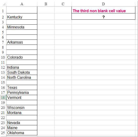
Введіть цю формулу: =INDEX($A$1:$A$25,SMALL(ROW($A$1:$A$25)+(100*($A$1:$A$25="")), 3))&"" у порожню комірку, де потрібно вивести результат, наприклад D2, а потім натисніть Ctrl + Shift + Enter клавіші разом, щоб отримати правильний результат, див. знімок екрана:

doc знайти n-ту непорожню 2

примітки: У наведеній вище формулі, A1: A25 - це список даних, який ви хочете використовувати, та номер 3 вказує значення третьої не пустої комірки, яку ви хочете повернути, якщо ви хочете отримати другу не пусту комірку, вам просто потрібно змінити число 3 на 2, як вам потрібно.


стрілка синя права міхур Знайдіть і поверніть n-те не пусте значення клітинки з рядка з формулою

Якщо ви хочете знайти і повернути n-те не пусте значення клітинки підряд, наступна формула може вам допомогти, зробіть так:

Введіть цю формулу: =INDEX($A$1:$M$1,SMALL(IF($A$1:$M$1<>"",COLUMN($A$1:$M$1)-COLUMN($A$1)+1),4)) у порожню клітинку, де потрібно знайти результат, а потім натисніть Ctrl + Shift + Enter клавіші разом, щоб отримати результат, див. скріншот:

doc знайти n-ту непорожню 3

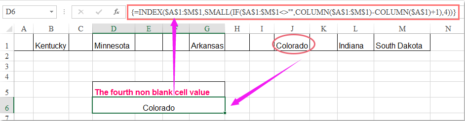
Примітка: У наведеній вище формулі A1: M1 - значення рядків, які ви хочете використовувати, і число 4 - це четверта не пуста клітинка, яку ви хочете повернути, якщо ви хочете отримати другу не пусту клітинку, вам просто потрібно змінити число 4 на 2, як вам потрібно.

Найкращі інструменти продуктивності офісу

🤖 Kutools AI Aide: Революціонізуйте аналіз даних на основі: Інтелектуальне виконання   |  Згенерувати код  |  Створення спеціальних формул  |  Аналізуйте дані та створюйте діаграми  |  Викликати функції Kutools...
Популярні функції: Знайдіть, виділіть або визначте дублікати   |  Видалити порожні рядки   |  Об’єднайте стовпці або клітинки без втрати даних   |   Раунд без Формули ...
Супер пошук: VLookup за кількома критеріями    Багатозначний VLookup  |   VLookup на кількох аркушах   |   Нечіткий пошук ....
Розширений розкривний список: Швидке створення випадаючого списку   |  Залежний спадний список   |  Виберіть розкривний список, що вибирається ....
Менеджер колонок: Додайте конкретну кількість стовпців  |  Перемістити стовпці  |  Перемкнути статус видимості прихованих стовпців  |  Порівняйте діапазони та стовпці ...
Особливості: Фокус сітки   |  Перегляд дизайну   |   Велика панель формул    Диспетчер робочих книг і аркушів   |  Бібліотека ресурсів (автотекст)   |  Вибір дати   |  Об’єднайте робочі аркуші   |  Шифрування/розшифрування клітинок    Надсилайте листи за списком   |  Супер фільтр   |   Спеціальний фільтр (фільтр жирний/курсив/закреслений...) ...
Топ-15 наборів інструментів12 текст Tools (додати текст, Видалити символи, ...)   |   50 + Графік типи (діаграма Ганта, ...)   |   40+ Практичний Формули (Розрахуйте вік на основі дня народження, ...)   |   19 вставка Tools (Вставте QR-код, Вставити зображення зі шляху, ...)   |   12 Перетворення Tools (Числа до слів, Валютна конверсія, ...)   |   7 Злиття та розділення Tools (Розширені комбіновані ряди, Розділені клітини, ...)   |   ... і більше

Покращуйте свої навички Excel за допомогою Kutools для Excel і відчуйте ефективність, як ніколи раніше. Kutools для Excel пропонує понад 300 додаткових функцій для підвищення продуктивності та економії часу.  Натисніть тут, щоб отримати функцію, яка вам найбільше потрібна...

Опис


Вкладка Office Передає інтерфейс із вкладками в Office і значно полегшує вашу роботу

  • Увімкніть редагування та читання на вкладках у Word, Excel, PowerPoint, Publisher, Access, Visio та Project.
  • Відкривайте та створюйте кілька документів на нових вкладках того самого вікна, а не в нових вікнах.
  • Збільшує вашу продуктивність на 50% та зменшує сотні клацань миші для вас щодня!
Comments (10)
No ratings yet. Be the first to rate!
This comment was minimized by the moderator on the site
CIAO STO CERCANDO DI APPLICARE LA TUA FORMULA MA NON MI FUNZIONA, DOVE STO SBAGLIANDO?
=INDICE($K$37:$K$88;MIN(RIGHE($K$37:$K$88)+RIGHE(100*($K$37:$K$88=""));6))&""
DEVO VISUALIZZARE L'ENNESIMA RIGA DIVERSA DA VUOTO

GRAzie
This comment was minimized by the moderator on the site
=INDICE($K$37:$K$88;MIN(RIGHE($K$37:$K$88)+(100*($K$37:$K$88=""));6))&""
This comment was minimized by the moderator on the site
I'm running this formula on a ~400 row sheet with around 20 blanks mixed throughout the data, and it's working perfectly EXCEPT when I fill the series down, it sometimes duplicates a row for some reason. For example, it seems to think a value is somehow simultaneously the 331st non-blank and the 332nd.

Things I've noticed:
-Duplications always happen in pairs (ex. 331 and 332 are duplicates, 333 and 334 will also be), then it goes back to normal for a while.
-Raw data also has blanks in pairs, but not corresponding to the duplicates
-No duplications occur in the first 94 rows, but they happen every 33-35 rows after that
-Does not appear to be linked to the value in the cell being duplicated
-I have entered as an array and as a standard formula, no difference in function

For reference, here's my actual formula:

=INDEX('PO Raw Data'!CR:CR,SMALL(ROW('PO Raw Data'!CR:CR)+(100*('PO Raw Data'!CR:CR="")),$W2)&"")

Note $W2 refers to a helper column and counts up as the data set is filled down, but only because I couldn't get it to count up when I just used a number instead of cell reference.
When I've replaced that cell reference (ex. $W2) with the appropriate number, same result.


Any thoughts on what I can do to fix that?
This comment was minimized by the moderator on the site
very helpful,
although when I return the nth non blank cell in a column set to DATE, the returned value appears as number(general number).formatting the cell into DATE also doesn't change the result. could you please give me a hand!
thanks a lot
This comment was minimized by the moderator on the site
Hello, Shirazi,
Sorry, maybe there is no direct formula for you to get the date format.

If someone else has the solution, please comment here.
This comment was minimized by the moderator on the site
Hi everyone!


Could you also help me return the row number of the second, third non-blank cell?


Please help me.
This comment was minimized by the moderator on the site
Hello, John,
the following formula can help you to get all the row numbers of the non-blank cells, please try it, thank you!
=IFERROR(ROW(INDEX($A$1:$A$12,SMALL(INDEX(NOT(ISBLANK($A$1:$A$12))*ROW($A$1:$A$12),0),COUNTBLANK($A$1:$A$12)+ROW(A1)))),"")
This comment was minimized by the moderator on the site
Hey everyone,

I have a table with numerous columns and rows. The rows have range names, and a description/location at the beginning of the row range with its own range, example "Building No.s". There are multiple Row Ranges/ Buildings. There are headers at the top of each columns for specific "Building Assembly Types". The table content is numeric quantities for each type "Building Assembly Type" for each specific "Building" description/location. There could be as many as (100) "Building Assembly Types" column headers but I will limit the assemblies to (10) per row range, so there will be numerous blank cells in each "Building No." range.

I have other summary tables set up for each "Building" that I want to pull the non-blank cells quantities to, along with the corresponding header "Assembly Type" for each "Building" with a (10) max "Assemblies" per page.

I can identify the non-blank cell quantities by use of the array formula above for rows. The problem I am having is identifying the header that corresponds to it.

Ultimately if I can identify the "Assembly" header, I can always index the "Quantities" once I have the header "Assembly" identified for each "Building". Then I would be able do a lookup for all the parts associated with each "Assembly" type for that "Building" from my Assembly parts database and multiply it times the "Quantity" of each assembly type.

Hopefully this makes since and someone can help.
This comment was minimized by the moderator on the site
Hello, I am looking for the third blank row in a column and I copied your formula and just changed the range from $A$1:$A:$25 to my range $D$306:$D$354. But when I change the range I get #REF! as my answer. I already converted to an array, control-shift-enter. Now the cell range I am referencing has formulas in them, so could that be why I am getting #REF. Your formula: =INDEX($A$1:$A$25,SMALL(ROW($A$1:$A$25)+(100*($A$1:$A$25="")), 3))&"" My formula: =INDEX($D$306:$D$354,SMALL(ROW($D$306:$D$354)+(1*($D$306:$D$354="")), 2))&"" Thanks, Noel
This comment was minimized by the moderator on the site
you have put the 1 instead of 100 therefore answered was wrong. please use below formula

INDEX($D$306:$D$354,SMALL(ROW($D$306:$D$354)+(100*($D$306:$D$354="")), 3))&"" than ctrl + shift+enter
There are no comments posted here yet
Please leave your comments in English
Posting as Guest
×
Rate this post:
0   Characters
Suggested Locations