Перейти до основного матеріалу

Як відобразити відповідну назву найвищого балу в Excel?

Припустимо, у мене є діапазон даних, який містить два стовпці - стовпець з іменем та відповідний стовпець з оцінками, тепер я хочу отримати ім’я людини, яка набрала найбільший бал. Чи є якісь хороші способи швидко вирішити цю проблему в Excel?

Відобразіть відповідну назву найвищого балу за допомогою формул


стрілка синя права міхур Відобразіть відповідну назву найвищого балу за допомогою формул

Щоб отримати ім’я особи, яка набрала найбільший бал, наступні формули можуть допомогти вам отримати результати.

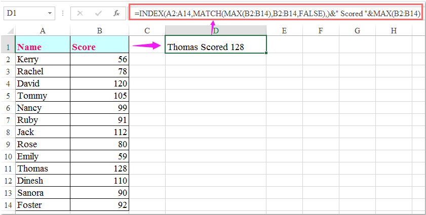
Введіть цю формулу: =INDEX(A2:A14,MATCH(MAX(B2:B14),B2:B14,FALSE),)&" Scored "&MAX(B2:B14) у порожню комірку, де потрібно відобразити ім’я, а потім натисніть Що натомість? Створіть віртуальну версію себе у клавіша для повернення результату наступним чином:

doc відображуване ім'я найвищий бал 1

Примітки:

1. У наведеній вище формулі A2: A14 - це список імен, з якого ви хочете отримати ім'я, та B2: B14 - це бальний список.

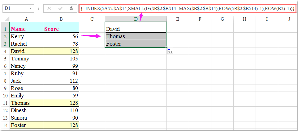
2. Вищевказана формула може отримати перше ім'я, лише якщо є кілька імен, що мають однакові найвищі оцінки. Щоб отримати всі імена, які отримали найвищий бал, наступна формула масиву може зробити вам послугу.

Введіть цю формулу:

=INDEX($A$2:$A$14,SMALL(IF($B$2:$B$14=MAX($B$2:$B$14),ROW($B$2:$B$14)-1),ROW(B2)-1)), а потім натисніть Ctrl + Shift + Enter клавіші разом, щоб відобразити перше ім'я, потім виберіть комірку формули і перетягніть маркер заповнення вниз, поки не з'явиться значення помилки, всі імена, які отримали найвищий бал, відображаються, як показано на знімку екрана:

doc відображуване ім'я найвищий бал 2

Найкращі інструменти продуктивності офісу

🤖 Kutools AI Aide: Революціонізуйте аналіз даних на основі: Інтелектуальне виконання   |  Згенерувати код  |  Створення спеціальних формул  |  Аналізуйте дані та створюйте діаграми  |  Викликати функції Kutools...
Популярні функції: Знайдіть, виділіть або визначте дублікати   |  Видалити порожні рядки   |  Об’єднайте стовпці або клітинки без втрати даних   |   Раунд без Формули ...
Супер пошук: VLookup за кількома критеріями    Багатозначний VLookup  |   VLookup на кількох аркушах   |   Нечіткий пошук ....
Розширений розкривний список: Швидке створення випадаючого списку   |  Залежний спадний список   |  Виберіть розкривний список, що вибирається ....
Менеджер колонок: Додайте конкретну кількість стовпців  |  Перемістити стовпці  |  Перемкнути статус видимості прихованих стовпців  |  Порівняйте діапазони та стовпці ...
Особливості: Фокус сітки   |  Перегляд дизайну   |   Велика панель формул    Диспетчер робочих книг і аркушів   |  Бібліотека ресурсів (автотекст)   |  Вибір дати   |  Об’єднайте робочі аркуші   |  Шифрування/розшифрування клітинок    Надсилайте листи за списком   |  Супер фільтр   |   Спеціальний фільтр (фільтр жирний/курсив/закреслений...) ...
Топ-15 наборів інструментів12 текст Tools (додати текст, Видалити символи, ...)   |   50 + Графік типи (діаграма Ганта, ...)   |   40+ Практичний Формули (Розрахуйте вік на основі дня народження, ...)   |   19 вставка Tools (Вставте QR-код, Вставити зображення зі шляху, ...)   |   12 Перетворення Tools (Числа до слів, Валютна конверсія, ...)   |   7 Злиття та розділення Tools (Розширені комбіновані ряди, Розділені клітини, ...)   |   ... і більше

Покращуйте свої навички Excel за допомогою Kutools для Excel і відчуйте ефективність, як ніколи раніше. Kutools для Excel пропонує понад 300 додаткових функцій для підвищення продуктивності та економії часу.  Натисніть тут, щоб отримати функцію, яка вам найбільше потрібна...

Опис


Вкладка Office Передає інтерфейс із вкладками в Office і значно полегшує вашу роботу

  • Увімкніть редагування та читання на вкладках у Word, Excel, PowerPoint, Publisher, Access, Visio та Project.
  • Відкривайте та створюйте кілька документів на нових вкладках того самого вікна, а не в нових вікнах.
  • Збільшує вашу продуктивність на 50% та зменшує сотні клацань миші для вас щодня!
Comments (17)
No ratings yet. Be the first to rate!
This comment was minimized by the moderator on the site
Hi sir, I tried this method, But the problem is if top two students have the same score when I look for the highest 3 one student's name alone is repeated twice with the same score instead of second student's name. How to solve this.
This comment was minimized by the moderator on the site
Hello, Divyanathan
Maybe the following array formula can help you:

=IFERROR(INDEX(A:A,SUM(IF(($B$2:$B$100+ROUND(0.1/ROW($B$2:$B$100),5))=LARGE($B$2:$B$100+ROUND(0.1/ROW($B$2:$B$100),5),ROW(A1)),ROW($B$2:$B$100)))),"")


Note: After inserting the formula, please press Ctrl + Shift + Enter keys together to get the first result, and then drga this formula cell down to get the largest n results as you need.

Please have a try, hope it can help you!
This comment was minimized by the moderator on the site
Hola disculpa me podrías apoyar para sacar la formula o otro tipo de dato que me pueda dar el nombre del tota de un resultado?

explico tengo una tabla con 4 nombres diferentes distribuidos en las celdas C3,D3,E3 y F3 de las cuales cada celda mencionada tiene rangos de productos ejemplo: detergentes
y cada celda mencionada tiene precios diferentes.
en el resultado que debo de mostrar es el valor mínimo de precio de cada detergente de las celdas ya mencionadas arriba, y a lo que quiero llegar es que indique una formula o un dato que indique que en cada resultado a la derecho me indique el nombre del valor de resultado.
muestro un ejemplo mas especifico: en la celda <C3> tiene un nombre de insumos, en la celda C4 hasta C120 están los precios de cada detergente que maneja la celda C3, en la celda <D3> esta un nombre de biodetergentes, y mismo proceso la celda D4 hasta D120 están los precios en la celda G4 se encuentra el resultado del valor mínimo de estos dos nombres (insumos-biodetergentes) teniendo el valor menor el de nombre de insumos. ahora en la celda H4 quiero que me aparezca el nombre del valor de resultado en este caso que me aparezca el nombre de "insumos" como puedo hacer para que me aparezca este nombre? espero me allá podido dar a entender de lo que requiero
muchas gracias por su atención
saludos cordiales.
This comment was minimized by the moderator on the site
ik heb het ook geprobeerd met alle dezelfde gegevens zoals in het voorbeeld maar het werkt totaal niet
This comment was minimized by the moderator on the site
Hello jac, Sorry to hear that. As I have answered in the below comment, the two formulas work great for me. And I have been wondering why the formulas aren't working for the readers. There are two reasons that can lead to the malfunction of the second formula. 
First, if you are using Excel versions before Excel 2020, then you must enter the formula =INDEX($A$2:$A$14,SMALL(IF($B$2:$B$14=MAX($B$2:$B$14),ROW($B$2:$B$14)-1),ROW(B2)-1)) via pressing Ctrl + Shift + Enter keys together.
Second, When you get the first result, remember to select the formula cell and drag the fill handle down until error value appears. So all the other results will be returned.
And as you can see in the screenshots below, the two formulas are working fine for me.  Hope my solution works. Have a nice day.
Sincerely,Mandy
This comment was minimized by the moderator on the site
bullshitdoes not work
This comment was minimized by the moderator on the site
Hello,
Sorry to hear that. But I did tried the two formulas in the article and both of them works perfectly. Please see the screenshots I uploaded here. And we would love to solve the problem for you if you can provide the details of the problem. Looking forward to your reply.Sincerely,Mandy
This comment was minimized by the moderator on the site
Trying to do the same thing but with the minimum score in Microsoft sheets. I swapped max for min as below and it didn't work =INDEX($A$2:$A$14,SMALL(IF($B$2:$B$14=MIN($B$2:$B$14),ROW($B$2:$B$14)-1),ROW(B2)-1))
This comment was minimized by the moderator on the site
Hi. This formula was exactly what I was looking for. However is there a way do this with the lowest Score but above 0 (in my case £00.00) I removed the bit of formula that displays the amount as only needed the Name and comment.I changed the MAX for MIN but there are a few entries at 0 (£00.00) and formula displays the name for the first of the '0' entries
This comment was minimized by the moderator on the site
Hello, Nigel,To lookup the lowest value above 0, you should apply the below array formula:After entering the formula, please remember to press Ctrl + Shift + Enter keys together to get the correct result.=INDEX(A2:A8,MATCH(MIN(IF(B2:B8>0,B2:B8)),B2:B8,0))&" Scored "&MIN(IF(B2:B8>0,B2:B8))
Please try, hope it can help you!
This comment was minimized by the moderator on the site
How do you find the second highest student? Please help me :( I only get the name of Thomas.
This comment was minimized by the moderator on the site
How do you find the second highest student?
This comment was minimized by the moderator on the site
How would you show two names if the high scores match?
This comment was minimized by the moderator on the site
Hello, Chris,
To get all names if there are multiple high scores match, the second formula in this article can do you a favor.
Please try it, thank you!
This comment was minimized by the moderator on the site
How would you get the matching numbers with the corresponding names to display horizontally?
There are no comments posted here yet
Load More
Please leave your comments in English
Posting as Guest
×
Rate this post:
0   Characters
Suggested Locations