Перейти до основного матеріалу

Як встановити / показати попередньо вибране значення для випадаючого списку в Excel?

За замовчуванням загальний розкривний список, який ви створили, відображається пустим, перш ніж вибрати одне значення зі списку, але в деяких випадках вам може знадобитися показати або встановити заздалегідь вибране значення / значення за замовчуванням для випадаючого списку, перш ніж користувачі виберуть його із список, як показано нижче. Тут ця стаття може вам допомогти.


стрілка синя права міхур Встановіть значення за замовчуванням (попередньо вибране значення) для випадаючого списку з формулою

Щоб встановити значення за замовчуванням для випадаючого списку, потрібно спочатку створити загальний випадаючий список, а потім використовувати формулу.

1. Створіть випадаючий список. Виділіть клітинку або діапазон, який ви хочете розмістити у випадаючому списку, ось K1, і натисніть дані > Перевірка достовірності даних. Дивіться знімок екрана:
doc показати попередньо вибране значення випадаючого списку 2

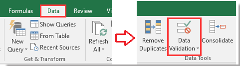
2. Потім у Перевірка достовірності даних діалогове вікно, під Налаштування вкладка, виберіть список від дозволяти , а потім виберіть значення, яке потрібно відобразити у спадному списку Source текстове вікно. Дивіться знімок екрана:
doc показати попередньо вибране значення випадаючого списку 3

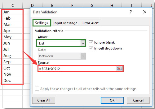
3 Потім натисніть Повідомлення про помилку Вкладка в Перевірка достовірності даних та зніміть прапорець Показувати попередження про помилку після введення недійсних даних варіант. див. скріншот:
doc показати попередньо вибране значення випадаючого списку 4

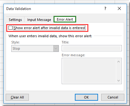
4. клацання OK щоб закрити діалогове вікно, перейдіть до випадаючого списку та введіть цю формулу = IF (J1 = "", "--select--") в неї та натисніть Що натомість? Створіть віртуальну версію себе у ключ. Дивіться знімок екрана:
doc показати попередньо вибране значення випадаючого списку 5

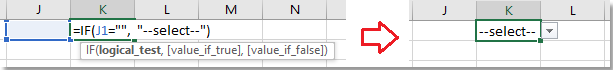
Порада: У формулі J1 - це порожня комірка поруч із K1, переконайтеся, що комірка порожня, і "--виберіть -"- це попередньо вибране значення, яке ви хочете показати, і ви можете змінювати їх, як вам потрібно.

5. Потім залиште клітинку випадаючого списку вибраною та натисніть дані > Перевірка достовірності даних , Щоб показати, Перевірка достовірності даних знову відкрийте діалогове вікно та перейдіть до Повідомлення про помилку та перевірте Показувати попередження про помилку після введення недійсних даних варіант назад. Дивіться знімок екрана:
doc показати попередньо вибране значення випадаючого списку 6

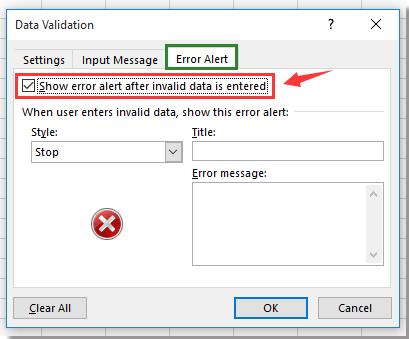
7. клацання OK, тепер перед тим, як користувачі вибирають значення зі спадного списку, у вказаній комірці зі спадним списком відображається значення за замовчуванням.
doc показати попередньо вибране значення випадаючого списку 7

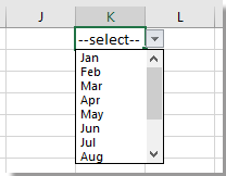
Примітка: Поки значення вибирається зі спадного списку, значення за замовчуванням зникає.
doc показати попередньо вибране значення випадаючого списку 8


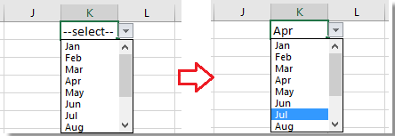
Найкращі інструменти продуктивності офісу

🤖 Kutools AI Aide: Революціонізуйте аналіз даних на основі: Інтелектуальне виконання   |  Згенерувати код  |  Створення спеціальних формул  |  Аналізуйте дані та створюйте діаграми  |  Викликати функції Kutools...
Популярні функції: Знайдіть, виділіть або визначте дублікати   |  Видалити порожні рядки   |  Об’єднайте стовпці або клітинки без втрати даних   |   Раунд без Формули ...
Супер пошук: VLookup за кількома критеріями    Багатозначний VLookup  |   VLookup на кількох аркушах   |   Нечіткий пошук ....
Розширений розкривний список: Швидке створення випадаючого списку   |  Залежний спадний список   |  Виберіть розкривний список, що вибирається ....
Менеджер колонок: Додайте конкретну кількість стовпців  |  Перемістити стовпці  |  Перемкнути статус видимості прихованих стовпців  |  Порівняйте діапазони та стовпці ...
Особливості: Фокус сітки   |  Перегляд дизайну   |   Велика панель формул    Диспетчер робочих книг і аркушів   |  Бібліотека ресурсів (автотекст)   |  Вибір дати   |  Об’єднайте робочі аркуші   |  Шифрування/розшифрування клітинок    Надсилайте листи за списком   |  Супер фільтр   |   Спеціальний фільтр (фільтр жирний/курсив/закреслений...) ...
Топ-15 наборів інструментів12 текст Tools (додати текст, Видалити символи, ...)   |   50 + Графік типи (діаграма Ганта, ...)   |   40+ Практичний Формули (Розрахуйте вік на основі дня народження, ...)   |   19 вставка Tools (Вставте QR-код, Вставити зображення зі шляху, ...)   |   12 Перетворення Tools (Числа до слів, Валютна конверсія, ...)   |   7 Злиття та розділення Tools (Розширені комбіновані ряди, Розділені клітини, ...)   |   ... і більше

Покращуйте свої навички Excel за допомогою Kutools для Excel і відчуйте ефективність, як ніколи раніше. Kutools для Excel пропонує понад 300 додаткових функцій для підвищення продуктивності та економії часу.  Натисніть тут, щоб отримати функцію, яка вам найбільше потрібна...

Опис


Вкладка Office Передає інтерфейс із вкладками в Office і значно полегшує вашу роботу

  • Увімкніть редагування та читання на вкладках у Word, Excel, PowerPoint, Publisher, Access, Visio та Project.
  • Відкривайте та створюйте кілька документів на нових вкладках того самого вікна, а не в нових вікнах.
  • Збільшує вашу продуктивність на 50% та зменшує сотні клацань миші для вас щодня!
Comments (15)
No ratings yet. Be the first to rate!
This comment was minimized by the moderator on the site
Hi,

How to count (D71) conditionally formatted RED color cell (D40:D70)?

Pls guide...

Thanks.
This comment was minimized by the moderator on the site
Hi,

How to make default value (UP) for certain range of column (C40:C70) only in the below code? Add what command?

Private Sub Worksheet_Change(ByVal Target As Range)
‘Updated by ARUN
Dim xObjV As Validation
On Error Resume Next
Set xObjV = Target.Validation
If xObjV.Type = xlValidateList Then
If IsEmpty(Target.Value) Then Target.Value = “UP”
End If
End Sub

Pls guide…

Thanks.
This comment was minimized by the moderator on the site
Try this code
Private Sub Worksheet_Change(ByVal Target As Range)
    'Updated by ExtendOffice
    Dim xObjV As Validation
    On Error Resume Next
    Set xObjV = Target.Validation
    
    'Check if the target is within C40:C70
    If Not Intersect(Target, Range("C40:C70")) Is Nothing Then
        If xObjV.Type = xlValidateList Then
            If IsEmpty(Target.Value) Then Target.Value = "UP"
        End If
    End If
End Sub
This comment was minimized by the moderator on the site
Hi,

Its working...

Thanks
This comment was minimized by the moderator on the site
Hello, How can I get defined value limit in excel dropdown menu, like I want to Enter Apple in product against three name and it should not put 4th entry and give error if i do so, any solution please.
This comment was minimized by the moderator on the site
Sorry, I do not understand your question, could you describe with more details or upload a file to describe it?
This comment was minimized by the moderator on the site
Hello, How can I get defined value limit in excel dropdown menu, like I want to Enter Apple in product against three name and it should not put 4th entry and give error if i do so, any soluition please.
This comment was minimized by the moderator on the site
hello, my data is about names and phone numbers. can make it if two names selected in one cells using data validations, the particular name which their name as selected, their phone numbers will be shown next to it.

help me!
This comment was minimized by the moderator on the site
Hello!

How can I set a data validation list such that if the drop down value in the cell is deleted, the cell will automatically show a default value (i.e. "-Select-")?

For example, I have a worksheet with multiple drop down lists that I want to show a default value of "-Select-" once the sheet is opened. A user will select values from the lists that will impact the result of calculations throughout the entire spreadsheet. A user may accidentally "delete" the cell contents of the lists. If this happens, rather than the cell becoming blank, I want the cell to show a default value of "-Select-". This scenario occurs in multiple random locations throughout the spreadsheet, not just in one localized place.

I was able to find the following VBA code so far, but it only applies the concept over a range, rather than just individual cells that contain drop down lists. The problem with what I have coded so far is that every single blank cell in the range ends up with "-Select-" in it. Some of the lists are in ranges, but some are also scattered throughout the sheet. The problem I'm having with my current code is that every single blank cell in the range ends up with "-Select-" in it. I'm trying to get this to apply over the entire worksheet to ONLY cells that are drop down lists.

Is what I'm trying to accomplish even possible?

Example file can be found here:
https://drive.google.com/file/d/1VoO8VgFs3IJ0ALwqfk0i8gt69UE4vEKW/view?usp=sharing

Example code:

Option Explicit

Private Sub Worksheet_Change(ByVal Target As Range)
Dim cel As Range
' If Target.Cells.Count > 1 Then Exit Sub 'turning this off allows multiple cells to be selected and deleted at the same time
If Not Intersect(Target, Range("f2:p17")) Is Nothing Then
For Each cel In Range("f2:p17")
Application.EnableEvents = False
If IsEmpty(cel.Value) Then cel.Value = "-Select-"
Next cel
End If
Application.EnableEvents = True
End Sub


Thanks in advance!
This comment was minimized by the moderator on the site
How can I set a data validation list such that if the drop down value in the cell is deleted, the cell will automatically show the a default value (i.e. "-Select-")?

For example, I have a worksheet with multiple drop down lists that I want to show a default value of "-Select-" once the sheet is opened. A user will select values from the lists that will impact the result of calculations throughout the entire spreadsheet. A user may accidentally "delete" the cell contents. If this happens, rather than the cell becoming blank, I want the cell to show a default value of "-Select-". This scenario occurs in multiple random locations throughout the spreadsheet, not just in one localized place.

I was able to come up with the following VBA code so far, but I've only figured out how to apply the concept over a range, rather than just cells that contain a drop down list. The problem with what I have coded so far is that every single blank cell in the range ends up with "-Select-" in it.

Option Explicit

Private Sub Worksheet_Change(ByVal Target As Range)
Dim cel As Range
' If Target.Cells.Count > 1 Then Exit Sub
If Not Intersect(Target, Range("f2:p17")) Is Nothing Then
For Each cel In Range("f2:p17")
Application.EnableEvents = False
If IsEmpty(cel.Value) Then cel.Value = "-Select-"
Next cel
End If
Application.EnableEvents = True
End Sub
This comment was minimized by the moderator on the site
The idea is nice, but my problem is that if the dropdown value is deleted, it doesn't revert to the default.
This comment was minimized by the moderator on the site
I also have the same issue , please reply if you solved it
This comment was minimized by the moderator on the site
Exactly!!! I'm having the same issue, have you found a solution?
This comment was minimized by the moderator on the site
You can insert the function in that specific cell using VBA, make sure you call the insert function when workbook is opening.
This comment was minimized by the moderator on the site
Only works if you speak VBA, not all of us code.
There are no comments posted here yet
Please leave your comments in English
Posting as Guest
×
Rate this post:
0   Characters
Suggested Locations