Перейти до основного матеріалу

Як округлити дату до попереднього або наступного конкретного робочого дня в Excel?

doc-round-to-previous-sonday-1
Іноді може знадобитися отримати попередній або наступний конкретний день тижня, наприклад неділю, на основі дати, як показано на знімку екрана зліва. У цьому посібнику наведено дві формули для легкої обробки цієї роботи в Excel.
Округлення дати до наступного конкретного дня тижня
Дата округлення до попереднього певного дня тижня

стрілка синя права міхур Округлена дата до наступного конкретного дня тижня

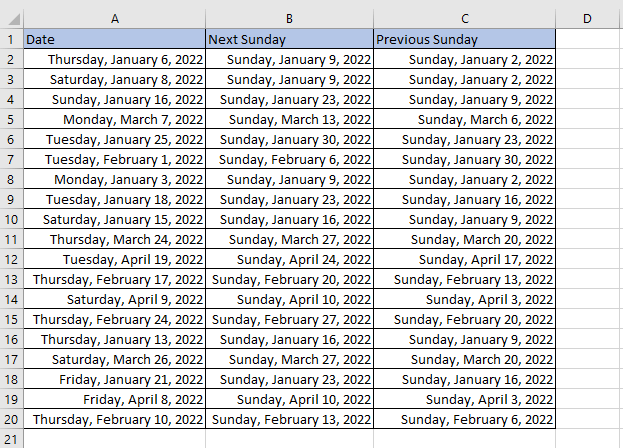
Наприклад, тут, щоб отримати наступну неділю з дат у стовпці A

1. Виберіть клітинку, в яку ви хочете розмістити наступну неділю, потім вставте або введіть формулу нижче:

=IF(MOD(A2-1,7)>7,A2+7-MOD(A2-1,7)+7,A2+7-MOD(A2-1,7))

2. Потім натисніть Що натомість? Створіть віртуальну версію себе у клавішу, щоб отримати першу наступну неділю, яка відображається як 5-значне число, потім перетягніть автоматичне заповнення вниз, щоб отримати всі результати.

doc-round-to-previous-sonday-1

3. Потім залишити виділеними клітинки формули, натисніть Ctrl + 1 клавіші для відображення Формат ячеек діалогове вікно, потім під Номер вкладка, виберіть Дата і виберіть один тип дати з правого списку, як вам потрібно. Натисніть OK.

doc-round-to-previous-sonday-1

Тепер результати формули відображаються у форматі дати.

doc-round-to-previous-sonday-1

Щоб отримати наступний інший день тижня, скористайтеся формулами нижче:

Weekday Formula
неділя =IF(MOD(A2-1,7)>7,A2+7-MOD(A2-1,7)+7,A2+7-MOD(A2-1,7))
Saturday =IF(MOD(A2-1,7)>6,A2+6-MOD(A2-1,7)+7,A2+6-MOD(A2-1,7))
п'ятниця =IF(MOD(A2-1,7)>5,A2+5-MOD(A2-1,7)+7,A2+5-MOD(A2-1,7))
четвер =IF(MOD(A2-1,7)>4,A2+4-MOD(A2-1,7)+7,A2+4-MOD(A2-1,7))
середа =IF(MOD(A1-1,7)>3,A1+3-MOD(A1-1,7)+7,A1+3-MOD(A1-1,7))
; вівторок =IF(MOD(A1-1,7)>2,A1+2-MOD(A1-1,7)+7,A1+2-MOD(A1-1,7))
понеділок =IF(MOD(A1-1,7)>1,A1+1-MOD(A1-1,7)+7,A1+1-MOD(A1-1,7))

стрілка синя права міхур Округлена дата до попереднього певного дня тижня

Наприклад, тут, щоб отримати попередню неділю з дат у стовпці A

1. Виберіть клітинку, в яку ви хочете розмістити наступну неділю, потім вставте або введіть формулу нижче:

=A2-ДЕНЬ ТИЖНЯ(A2,2)

2. Потім натисніть Що натомість? Створіть віртуальну версію себе у клавішу, щоб отримати першу наступну неділю, потім перетягніть автозаповнення вниз, щоб отримати всі результати.

doc-round-to-previous-sonday-1

Якщо ви хочете змінити формат дати, залишайте клітинки формули виділеними, натисніть Ctrl + 1 клавіші для відображення Формат ячеек діалогове вікно, потім під Номер вкладка, виберіть Дата і виберіть один тип дати з правого списку, як вам потрібно. Натисніть OK.

doc-round-to-previous-sonday-1

Тепер результати формули відображаються у форматі дати.

doc-round-to-previous-sonday-1

Щоб отримати попередній інший день тижня, скористайтеся наведеними нижче формулами:

Weekday Formula
неділя =A2-ДЕНЬ ТИЖНЯ(A2,2)
Saturday =IF(WEEKDAY(A2,2)>6,A2-WEEKDAY(A2,1),A2-WEEKDAY(A2,2)-1)
п'ятниця =IF(WEEKDAY(A2,2)>5,A2-WEEKDAY(A2,2)+5,A2-WEEKDAY(A2,2)-2)
четвер =IF(WEEKDAY(A2,2)>4,A2-WEEKDAY(A2,2)+4,A2-WEEKDAY(A2,2)-3)
середа =IF(WEEKDAY(A2,2)>3,A2-WEEKDAY(A2,2)+3,A2-WEEKDAY(A2,2)-4)
; вівторок =IF(WEEKDAY(A2,2)>2,A2-WEEKDAY(A2,2)+2,A2-WEEKDAY(A2,2)-5)
понеділок =IF(WEEKDAY(A2,2)>1,A2-WEEKDAY(A2,2)+1,A2-WEEKDAY(A2,2)-6)

Потужний помічник дати та часу

Команда Помічник дати та часу особливість Kutools для Excel, підтримує легко додавати/віднімати час дати, обчислювати різницю між двома датами та обчислювати вік на основі дня народження.  Клацніть на безкоштовну пробну версію!
doc-round-to-previous-sonday-1
 
Kutools для Excel: з більш ніж 200 зручними надбудовами Excel, які можна безкоштовно спробувати без обмежень.

Найкращі інструменти продуктивності офісу

🤖 Kutools AI Aide: Революціонізуйте аналіз даних на основі: Інтелектуальне виконання   |  Згенерувати код  |  Створення спеціальних формул  |  Аналізуйте дані та створюйте діаграми  |  Викликати функції Kutools...
Популярні функції: Знайдіть, виділіть або визначте дублікати   |  Видалити порожні рядки   |  Об’єднайте стовпці або клітинки без втрати даних   |   Раунд без Формули ...
Супер пошук: VLookup за кількома критеріями    Багатозначний VLookup  |   VLookup на кількох аркушах   |   Нечіткий пошук ....
Розширений розкривний список: Швидке створення випадаючого списку   |  Залежний спадний список   |  Виберіть розкривний список, що вибирається ....
Менеджер колонок: Додайте конкретну кількість стовпців  |  Перемістити стовпці  |  Перемкнути статус видимості прихованих стовпців  |  Порівняйте діапазони та стовпці ...
Особливості: Фокус сітки   |  Перегляд дизайну   |   Велика панель формул    Диспетчер робочих книг і аркушів   |  Бібліотека ресурсів (автотекст)   |  Вибір дати   |  Об’єднайте робочі аркуші   |  Шифрування/розшифрування клітинок    Надсилайте листи за списком   |  Супер фільтр   |   Спеціальний фільтр (фільтр жирний/курсив/закреслений...) ...
Топ-15 наборів інструментів12 текст Tools (додати текст, Видалити символи, ...)   |   50 + Графік типи (діаграма Ганта, ...)   |   40+ Практичний Формули (Розрахуйте вік на основі дня народження, ...)   |   19 вставка Tools (Вставте QR-код, Вставити зображення зі шляху, ...)   |   12 Перетворення Tools (Числа до слів, Валютна конверсія, ...)   |   7 Злиття та розділення Tools (Розширені комбіновані ряди, Розділені клітини, ...)   |   ... і більше

Покращуйте свої навички Excel за допомогою Kutools для Excel і відчуйте ефективність, як ніколи раніше. Kutools для Excel пропонує понад 300 додаткових функцій для підвищення продуктивності та економії часу.  Натисніть тут, щоб отримати функцію, яка вам найбільше потрібна...

Опис


Вкладка Office Передає інтерфейс із вкладками в Office і значно полегшує вашу роботу

  • Увімкніть редагування та читання на вкладках у Word, Excel, PowerPoint, Publisher, Access, Visio та Project.
  • Відкривайте та створюйте кілька документів на нових вкладках того самого вікна, а не в нових вікнах.
  • Збільшує вашу продуктивність на 50% та зменшує сотні клацань миші для вас щодня!
Comments (16)
No ratings yet. Be the first to rate!
This comment was minimized by the moderator on the site
I have tested this but partially incorrect result was out. Why ?
I wanted to get next Friday.

=IF(A2="","",A2+5-Mod(A2-1,7))

I have entered 11/19/2022
The result was past day 11/18/2022
This comment was minimized by the moderator on the site
Thanks for your reminder, the original formula is not enough rigorous indeed. I have updated the formulas and rewrited the tutorial, hope the new formulas can help you.
This comment was minimized by the moderator on the site
Im trying to work out how to use a date, less an amount of days but ensure when subtracting the days it lands on a weekday not a weekend.
Any formulas??
This comment was minimized by the moderator on the site
Hi Everyone,
I use the formula below to round to the next Thursday where A1 is the cell with your original date and 14 is for Thursday. You can use other numbers for other days if required. 11=Monday, 12=Tuesday, 13=Wednesday, etc...

Also, you can use a 1 instead of an 8 to get the Thursday before your original date in A1. If your original date is already a Thursday the formula will produce the same date as in A1.

I hope this helps!

=A1+(0-WEEKDAY(A1,14)+8)
This comment was minimized by the moderator on the site
Thank you! This worked :)
This comment was minimized by the moderator on the site
I put this into google sheets and to make the dates become next thursday but I have not been able to get it to work especially for the dates right after thursdays. =IF(L2="","",L2+4-MOD(L2-1,4)) is the function i used to make it thursday but not all dates were thursday.
This comment was minimized by the moderator on the site
to clarify, all dates become thursday, but friday and saturday will not convert to the next weeks thursday instead they will go back a day or two to the previous thursday instead going to next weeks thursday, is there any way to fix this in the function =IF(L4="","",L4+4-MOD(L4-1,7))
This comment was minimized by the moderator on the site
Hi Kisho,

I use the formula below to round to the next Thursday where A1 is the cell with your original date and 14 is for Thursday. You can use other numbers for other days if required. 11=Monday, 12=Tuesday, 13=Wednesday, etc...

Also, you can use a 1 instead of an 8 to get the Thursday before your original date in A1. If your original date is already a Thursday the formula will produce the same date as in A1.

I hope this helps!

=A1+(0-WEEKDAY(A1,14)+8)
This comment was minimized by the moderator on the site
Hi Kisho,
I use the formula below to round to the next Thursday where A1 is the cell with your original date and 14 is for Thursday. You can use other numbers for other days if required. 11=Monday, 12=Tuesday, 13=Wednesday, etc...
Also, you can use a 1 instead of an 8 to get the Thursday before your original date in A1. If your original date is already a Thursday the formula will produce the same date as in A1.
I hope this helps!
=A1+(0-WEEKDAY(A1,14)+8)
This comment was minimized by the moderator on the site
I put this into google sheets and to make the dates become next thursday but I have not been able to get it to work especially for the dates right after thursdays. =IF(L2="","",L2+4-MOD(L2-1,4)) is the function i used to make it thursday but not all dates were thursday.
This comment was minimized by the moderator on the site
Si quiero la fecha del próximo viernes cómo debo modificar las variables? Gracias
This comment was minimized by the moderator on the site
Sorry, I cannot understand, could you speak in English?
This comment was minimized by the moderator on the site
hi guys,

I used the formula below, I hope it works for you.
IF(WEEKDAY(H2,16)<>7,(7-WEEKDAY(H2,16))+H2,H2) where H2 is the date that you want to round up to the next day of the week (in my case for Friday) and the 16 is the format to start the date with Saturday as #1 and Friday as #7.
This comment was minimized by the moderator on the site
Your round to previous Sunday is flawed. Even shows as much on your sheet.
This comment was minimized by the moderator on the site
So, what would be the correct formula to first check to see if a cell has a date, else leave it blank and make the date the fall on a Friday before if the date falls on a Saturday or Sunday?
This comment was minimized by the moderator on the site
I found a workaround for to the previous Friday. You can change the switch "results" as needed to round to different days.=H3-SWITCH(TEXT(H3, "DDD"), "Mon", 3, "Tue", 4, "Wed", 5, "Thu", 6, "Fri", 0, "Sat", 1, "Sun", 2)
=[date]-SWITCH(TEXT([date], "DDD"), "Mon", 3, "Tue", 4, "Wed", 5, "Thu", 6, "Fri", 0, "Sat", 1, "Sun", 2)
There are no comments posted here yet
Please leave your comments in English
Posting as Guest
×
Rate this post:
0   Characters
Suggested Locations