Перейти до основного матеріалу

Як знайти першу або останню п’ятницю кожного місяця в Excel?

Зазвичай п’ятниця - останній робочий день місяця. Як можна знайти першу або останню п’ятницю на основі заданої дати в Excel? У цій статті ми проведемо вас, як використовувати дві формули для пошуку першої чи останньої п’ятниці кожного місяця.

Знайдіть першу п’ятницю місяця
Знайдіть останню п’ятницю місяця


Знайдіть першу п’ятницю місяця

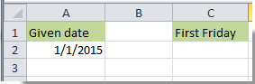
Наприклад, є дана дата, яку 1/1/2015 буде знаходити в комірці А2, як показано на знімку екрана нижче. Якщо ви хочете знайти першу п’ятницю місяця за даною датою, будь-ласка, зробіть наступне.

1. Виберіть клітинку для відображення результату. Тут ми обираємо клітинку С2.

2. Скопіюйте та вставте в неї формулу нижче, а потім натисніть Що натомість? Створіть віртуальну версію себе у ключ

=CEILING(EOMONTH(A2,-1)-5,7)+6

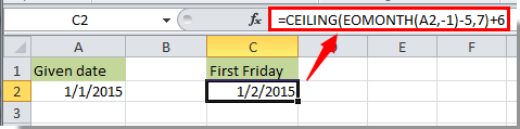
Потім дата відображається в комірці С2, це означає, що перша п’ятниця січня 2015 року є датою 1/2/2015.

примітки:

1. Якщо ви хочете знайти першу п’ятницю інших місяців, введіть вказану дату цього місяця в клітинку A2, а потім скористайтеся формулою.

2. У формулі A2 є еталонною коміркою, яку знаходить дана дата. Ви можете змінити його відповідно до своїх потреб.

Знайдіть останню п’ятницю місяця

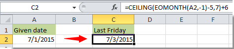
Вказана дата 1/1/2015 знаходиться в комірці A2, щоб знайти останню п’ятницю цього місяця в Excel, будь-ласка, виконайте наступні дії.

1. Виділіть комірку, скопіюйте в неї формулу нижче, а потім натисніть Що натомість? Створіть віртуальну версію себе у ключ, щоб отримати результат.

=DATE(YEAR(A2),MONTH(A2)+1,0)+MOD(-WEEKDAY(DATE(YEAR(A2),MONTH(A2)+1,0),2)-2,-7)

Потім в останню п’ятницю січня 2015 року відображається комірка В2.

примітки: Ви можете змінити A2 у формулі на еталонну комірку вказаної дати.


Статті по темі:

Найкращі інструменти продуктивності офісу

🤖 Kutools AI Aide: Революціонізуйте аналіз даних на основі: Інтелектуальне виконання   |  Згенерувати код  |  Створення спеціальних формул  |  Аналізуйте дані та створюйте діаграми  |  Викликати функції Kutools...
Популярні функції: Знайдіть, виділіть або визначте дублікати   |  Видалити порожні рядки   |  Об’єднайте стовпці або клітинки без втрати даних   |   Раунд без Формули ...
Супер пошук: VLookup за кількома критеріями    Багатозначний VLookup  |   VLookup на кількох аркушах   |   Нечіткий пошук ....
Розширений розкривний список: Швидке створення випадаючого списку   |  Залежний спадний список   |  Виберіть розкривний список, що вибирається ....
Менеджер колонок: Додайте конкретну кількість стовпців  |  Перемістити стовпці  |  Перемкнути статус видимості прихованих стовпців  |  Порівняйте діапазони та стовпці ...
Особливості: Фокус сітки   |  Перегляд дизайну   |   Велика панель формул    Диспетчер робочих книг і аркушів   |  Бібліотека ресурсів (автотекст)   |  Вибір дати   |  Об’єднайте робочі аркуші   |  Шифрування/розшифрування клітинок    Надсилайте листи за списком   |  Супер фільтр   |   Спеціальний фільтр (фільтр жирний/курсив/закреслений...) ...
Топ-15 наборів інструментів12 текст Tools (додати текст, Видалити символи, ...)   |   50 + Графік типи (діаграма Ганта, ...)   |   40+ Практичний Формули (Розрахуйте вік на основі дня народження, ...)   |   19 вставка Tools (Вставте QR-код, Вставити зображення зі шляху, ...)   |   12 Перетворення Tools (Числа до слів, Валютна конверсія, ...)   |   7 Злиття та розділення Tools (Розширені комбіновані ряди, Розділені клітини, ...)   |   ... і більше

Покращуйте свої навички Excel за допомогою Kutools для Excel і відчуйте ефективність, як ніколи раніше. Kutools для Excel пропонує понад 300 додаткових функцій для підвищення продуктивності та економії часу.  Натисніть тут, щоб отримати функцію, яка вам найбільше потрібна...

Опис


Вкладка Office Передає інтерфейс із вкладками в Office і значно полегшує вашу роботу

  • Увімкніть редагування та читання на вкладках у Word, Excel, PowerPoint, Publisher, Access, Visio та Project.
  • Відкривайте та створюйте кілька документів на нових вкладках того самого вікна, а не в нових вікнах.
  • Збільшує вашу продуктивність на 50% та зменшує сотні клацань миші для вас щодня!
Comments (12)
Rated 5 out of 5 · 1 ratings
This comment was minimized by the moderator on the site
Even shorter 😅
=lambda(Date;WeekDay;EOMONTH(Date;0)-WEEKDAY(EOMONTH(Date;0);WeekDay+10)+1
Where "WeekDay" parameter is 1=Monday, 7=Sunday
This comment was minimized by the moderator on the site
=lambda(Date;WeekDay;EOMONTH(Date;0)-WEEKDAY(EOMONTH(Date;0);WeekDay+10)+1)

I forgot a bracket at the end
This comment was minimized by the moderator on the site
Vậy công thức tính thứ sáu tuần thứ 2 của tháng như thế nào vậy ban?
This comment was minimized by the moderator on the site
Hi Tâm Cao Điền,
Suppose you want to calculate the second friday of the month based on the given date in A1, you can try the following formula:
=A18-DAY(A18)+CHOOSE(WEEKDAY(A18-DAY(A18),2),11,10,9,8,14,13,12)
This comment was minimized by the moderator on the site
porque cuando lo pruebo tal cual me sale error ?
o sea estoy copiando y pegando y no funciona

alguien sabe?
This comment was minimized by the moderator on the site
Hi andre,
Can you tell me which formula you used in the post? And what error your are experiencing?
This comment was minimized by the moderator on the site
Why not make the "last Friday" formula: =CEILING(EOMONTH(A2,0)-5,7)-1? That works for all dates I have tried....
This comment was minimized by the moderator on the site
Hi Eric,
I hop you are still on this forum and receive my reply.
Thanks so much for an EASY formula. I've never encountered =CEILING.
Rated 5 out of 5
This comment was minimized by the moderator on the site
Hi Eric,
Thanks for sharing it.
This comment was minimized by the moderator on the site
Hello and thank you for this formula. I am not an Excel guru and acnnot easily work out how to change this formula for the last Friday to be the Last Monday, or any other day. Can you please explain how to interpret this.
This comment was minimized by the moderator on the site
Matt,

The way the formula works is: First we find the last day of the month with the EOMONTH() function. For the last day of the current month, we use "0" as the month offset. For the previous month, it would be -1. (Either "=EOMONTH(A2,0)" or "=EOMONTH(A2,-1)".)

Then, in the "=CEILING()" function, we subtract the number of days required to bring us back to Sunday from the day for which we are searching. (For Tuesday, it would be -2, so we make the formula so far: "=CEILING(EOMONTH(A2,0)-2...."

We use the "significance" value of "7" because weeks are seven days long (of course).This finds the date of either the previous Saturday, or the following Saturday (Excel dates started with 1/1/1900, which was a Sunday. So if you enter a "1" in cell A2 with the Long Date format, the cell would read: "Sunday, January 1, 1900".). For that reason, the =CEILING() function, using "7" as the "significance" argument returns Saturday, which is always a multiple of 7 in Excel. Now the formula is "=CEILING(EOMONTH(A2,0)-2,7...".

Now we need to return the date to a Tuesday, so we either subtract 4 for the last Tuesday of the month, or add 3 for the first Tuesday of the next month. So the final formula is, respectively, either "=CEILING(EOMONTH(A2,0)-2,7)-4" or "=CEILING(EOMONTH(A2,0)-2,7)+3".

We can work through the math by assuming the last day of the month is either a Monday (assume its value is 9 - for ease of illustration, so the values do not go negative) or a Wednesday (assume value 11). "EOMONTH()" will return either of those days (9 or 11). Subtracting 2 results in the previous Saturday (value 7) or Monday (value 9), respectively. The CEILING() function then returns, respectively, the previous Saturday (value 7, because the ceiling of 7 with significance 7 is 7) or the current Saturday (value 14, because the ceiling of 9, significance 7, is 14). Subtracting 4 results in the previous Tuesday (value 3) or the current week's Tuesday (value 10), respectively. For the first Tuesday of the following month, adding 3 to the Saturday value (7 or 14) returns either Tuesday value 10, or Tuesday value 17, respectively.


Hopefully that helps you understand so that you can modify the formula as necessary. You can even change it to find the second Tuesday, or second to last Tuesday, by adding or subtracting an additional 7, respectively.
This comment was minimized by the moderator on the site
Hi Matt,
You just need to change the last number -7 to -1 to solove the problem.
=DATE(YEAR(A2),MONTH(A2)+1,0)+MOD(-WEEKDAY(DATE(YEAR(A2),MONTH(A2)+1,0),2)-2,-1)
There are no comments posted here yet
Please leave your comments in English
Posting as Guest
×
Rate this post:
0   Characters
Suggested Locations